options(repr.plot.width = 12, repr.plot.height = 6)EX 8.7 모의 실험 데이터
getwd()
'/home/coco/Dropbox/Scribbling/posts'
z <- scan("eg8_7.txt")
forecast::tsdisplay(z)
Registered S3 method overwritten by 'quantmod':
method from
as.zoo.data.frame zoo
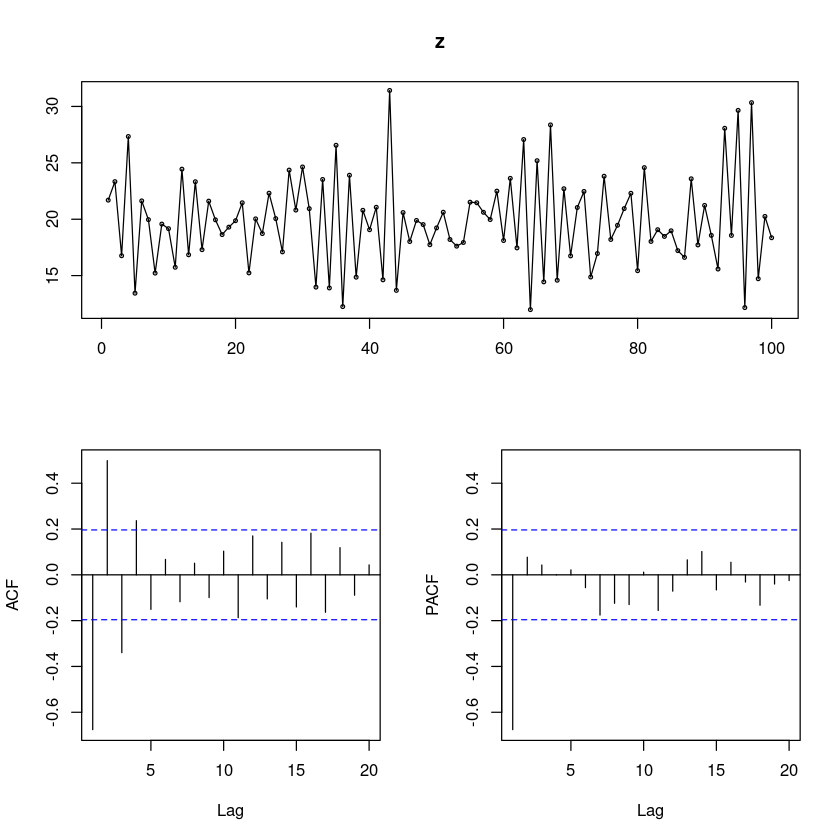
- 평균이 20정도로 움직이는 정상 시계열로 보인다. —> AR(1)모형
forecast::ggtsdisplay(z,
        smooth=T)
`geom_smooth()` using formula = 'y ~ x'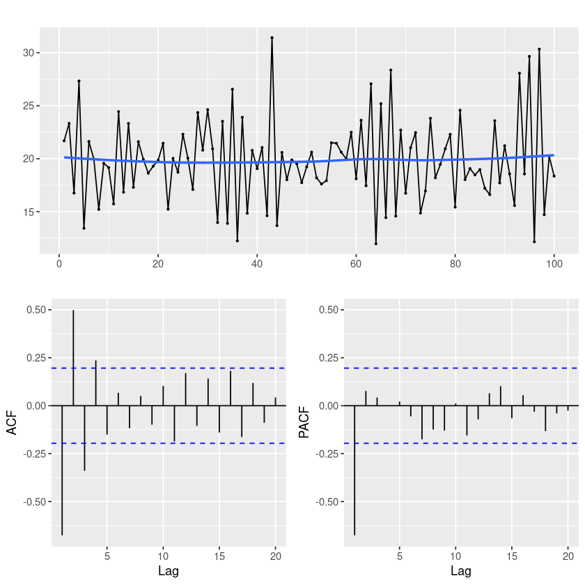
smooth=T를 쓰면 추세가 있는지 확인하는 파란 선이 생긴다.
fit <- arima(z, order=c(1,0,0), method='ML')
fit
Call:
arima(x = z, order = c(1, 0, 0), method = "ML")

Coefficients:
          ar1  intercept
      -0.6715    19.8312
s.e.   0.0728     0.1776

sigma^2 estimated as 8.744: log likelihood = -250.61, aic = 507.22mean(z)
19.832691
intercept는 delta가 아니라 mu이다.
\(\hat Z_n(l) = \hat μ + \hat ϕ^l(Z_n − \hat μ)\)
length(z)
100
- 예측하는 함수
- 모형을 기준으로 25개를 예측할거야!
forecast_fit <- forecast::forecast(fit, 25) #MMSE : zn(l) = mu + phi^l*(zn-mu), l=1,...,25
forecast_fit
Point Forecast Lo 80 Hi 80 Lo 95 Hi 95
101 20.82225 17.03269 24.61181 15.02662 26.61788
102 19.16558 14.60082 23.73034 12.18439 26.14678
103 20.27811 15.40393 25.15229 12.82369 27.73253
104 19.53100 14.52353 24.53847 11.87273 27.18926
105 20.03272 14.96628 25.09915 12.28427 27.78116
106 19.69579 14.60299 24.78859 11.90702 27.48456
107 19.92205 14.81740 25.02670 12.11517 27.72893
108 19.77011 14.66013 24.88009 11.95507 27.58515
109 19.87214 14.75976 24.98453 12.05343 27.69086
110 19.80362 14.69015 24.91709 11.98325 27.62399
111 19.84964 14.73568 24.96359 12.02852 27.67076
112 19.81874 14.70456 24.93291 11.99728 27.64019
113 19.83949 14.72521 24.95376 12.01788 27.66110
114 19.82555 14.71123 24.93987 12.00387 27.64723
115 19.83491 14.72057 24.94925 12.01320 27.65662
116 19.82863 14.71428 24.94297 12.00690 27.65035
117 19.83285 14.71849 24.94720 12.01112 27.65457
118 19.83001 14.71566 24.94437 12.00828 27.65174
119 19.83191 14.71756 24.94627 12.01018 27.65365
120 19.83064 14.71628 24.94499 12.00890 27.65237
121 19.83150 14.71714 24.94585 12.00976 27.65323
122 19.83092 14.71656 24.94527 12.00919 27.65265
123 19.83131 14.71695 24.94566 12.00957 27.65304
124 19.83105 14.71669 24.94540 12.00931 27.65278
125 19.83122 14.71686 24.94558 12.00949 27.65295- 직접 계산
coef(fit)- ar1
- -0.671544059932036
- intercept
- 19.8311503070686
hat_phi <- coef(fit)[1]
hat_mu <- coef(fit)[2]
hat_mu + hat_phi * (z[100] - hat_mu) # l= 1 z_100_(1)
hat_mu + hat_phi^2 * (z[100] - hat_mu) # l= 2 z_100_(2)
intercept: 20.8222488141294
intercept: 19.1655839918444
- 100번째를 기준으로 그 다음값을 구하고 싶어.
l <- 1:10
sapply(l, function(x) hat_mu + hat_phi^x * (z[100] - hat_mu))- intercept
- 20.8222488141294
- intercept
- 19.1655839918444
- intercept
- 20.2781074125482
- intercept
- 19.5309989178393
- intercept
- 20.0327151895859
- intercept
- 19.6957906075232
- intercept
- 19.9220503092525
- intercept
- 19.7701069505542
- intercept
- 19.8721436105341
- intercept
- 19.8036214976293
plot(forecast_fit)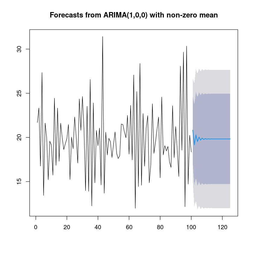
점점 평균값으로 수렴한다.
AR process의 정보가 점점 사라지는 것..
ggplot2::autoplot(forecast_fit)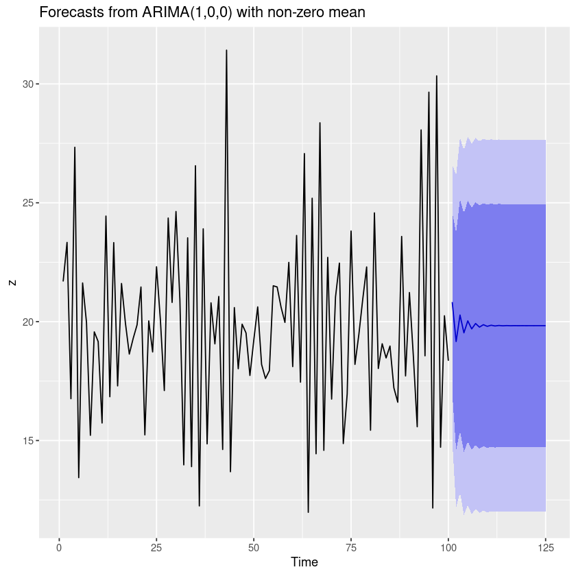
sarima_fit <- astsa::sarima.for(z,25,1,0,0) # z함수, 25개 볼거야, p, d, q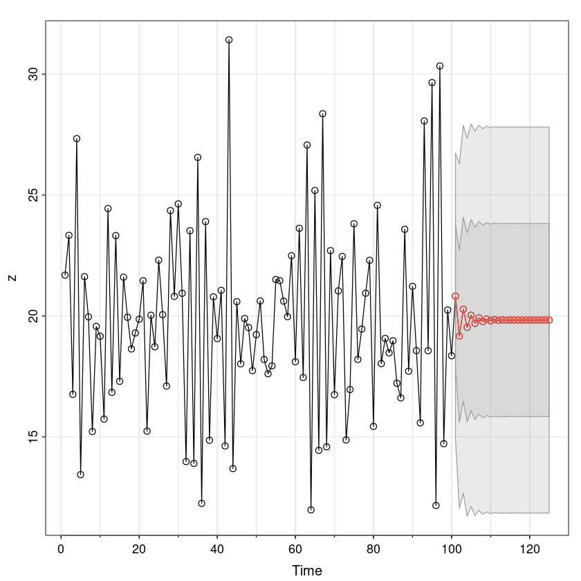
sarima_fit$pred
sarima_fit$se
A Time Series:
- 20.8222483489762
- 19.1655839559512
- 20.2781070098918
- 19.5309988141942
- 20.032714849742
- 19.6957904500696
- 19.9220500133516
- 19.7701067583474
- 19.8721433414928
- 19.8036212850204
- 19.849636861772
- 19.8187353767205
- 19.8394870839858
- 19.8255513992216
- 19.8349098248857
- 19.8286252301641
- 19.8328456121207
- 19.830011439887
- 19.8319147112811
- 19.8306365807722
- 19.8314949016627
- 19.8309185014078
- 19.8313055795478
- 19.8310456395405
- 19.831220200696
A Time Series:
- 2.95700711959937
- 3.5619005566917
- 3.80334404182832
- 3.90734998536685
- 3.95335857242263
- 3.97393285636323
- 3.98317649989949
- 3.98733810739122
- 3.98921345277822
- 3.99005889146209
- 3.99044010149264
- 3.9906120043846
- 3.99068952524303
- 3.99072448443737
- 3.99074024993262
- 3.99074735969909
- 3.990750565996
- 3.99075201194324
- 3.99075266402387
- 3.99075295809352
- 3.9907530907105
- 3.99075315051696
- 3.99075317748796
- 3.99075318965111
- 3.99075319513634
head(sarima_fit$pred + qnorm(0.975)*sarima_fit$se) ##95% 신뢰구간 상한
head(sarima_fit$pred - qnorm(0.975)*sarima_fit$se) ##95% 신뢰구간 하한
A Time Series:
- 26.6178758054195
- 26.1467807635801
- 27.7325243526903
- 27.1892640605063
- 27.781155269663
- 27.4845557255219
A Time Series:
- 15.0266208925329
- 12.1843871483223
- 12.8236896670933
- 11.8727335678821
- 12.2842744298209
- 11.9070251746172
EX 9.5 IMA(1,1) = ARIMA(0,1,1)
- 차분을 했더니 MA(1)모형
z <- scan("eg9_5.txt")
forecast::ggtsdisplay(z, smooth=T)
`geom_smooth()` using formula = 'y ~ x'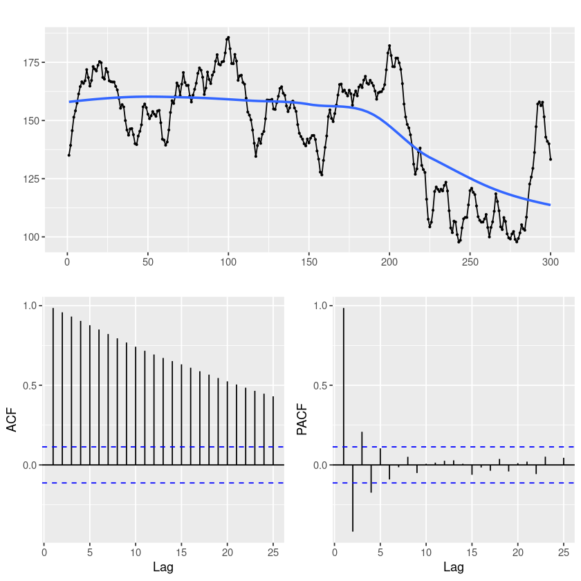
- ACF가 천천히 감소한다. (확률적 추세가 있어보임)
##단위근 검정 : H0 : 단위근이 있다.
fUnitRoots::adfTest(z, lags = 0, type = "c")
fUnitRoots::adfTest(z, lags = 1, type = "c")
fUnitRoots::adfTest(z, lags = 2, type = "c")
Title:
 Augmented Dickey-Fuller Test

Test Results:
  PARAMETER:
    Lag Order: 0
  STATISTIC:
    Dickey-Fuller: -1.43
  P VALUE:
    0.5246

Description:
 Tue Dec  5 20:19:59 2023 by user:
Title:
 Augmented Dickey-Fuller Test

Test Results:
  PARAMETER:
    Lag Order: 1
  STATISTIC:
    Dickey-Fuller: -2.3543
  P VALUE:
    0.1803

Description:
 Tue Dec  5 20:19:59 2023 by user:
Title:
 Augmented Dickey-Fuller Test

Test Results:
  PARAMETER:
    Lag Order: 2
  STATISTIC:
    Dickey-Fuller: -1.7307
  P VALUE:
    0.4126

Description:
 Tue Dec  5 20:19:59 2023 by user:
평균이 있으니 ‘C’ 옵션을 사용하자.
모든 차수에 대해서 p-value < 0.05이므로 차분이 필요하다.
lag_z <- diff(z)
forecast::tsdisplay(lag_z)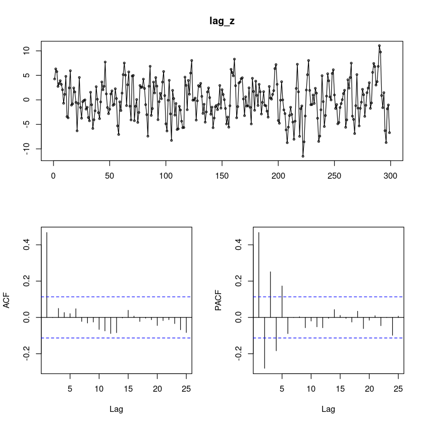
0을 중심으로 움직인다.
PACF가 SIN함수를 그리며 지수적으로 감소함
ACF가 1차에만 유효하고 나머지는 유효하지 않음 -> MA(1)모형
## mean : H0 : mu = 0
t.test(lag_z)
    One Sample t-test

data:  lag_z
t = -0.02617, df = 298, p-value = 0.9791
alternative hypothesis: true mean is not equal to 0
95 percent confidence interval:
 -0.4480209  0.4362617
sample estimates:
   mean of x
-0.005879599 - 유의확률이 크게 나와서 평균이 0이 맞아!
- 차분한 모형(평균 F)
fit1 <- arima(lag_z, order=c(0,0,1), include.mean = F)
fit1
Call:
arima(x = lag_z, order = c(0, 0, 1), include.mean = F)

Coefficients:
         ma1
      0.7605
s.e.  0.0342

sigma^2 estimated as 9.479:  log likelihood = -760.93,  aic = 1525.86
- 원래 모형(평균 있음)
fit <- arima(z, order=c(0,1,1))
fit
Call:
arima(x = z, order = c(0, 1, 1))

Coefficients:
         ma1
      0.7605
s.e.  0.0342

sigma^2 estimated as 9.479: log likelihood = -760.93, aic = 1525.86- 두 가지 방법이 모두 동일하게 나온다.
\(Z_t = ε_t + 0.7605ε_t, \hat θ = −0.7605\)
부호가 반대!!!
MA모형 평균이 없당
- 잔차분석
forecast::checkresiduals(fit)
    Ljung-Box test

data:  Residuals from ARIMA(0,1,1)
Q* = 7.1117, df = 9, p-value = 0.6255

Model df: 1.   Total lags used: 10
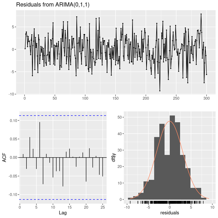
정규분포
10개시차까지 모든 cov가 0
WN이다
resid = resid(fit)
forecast::tsdisplay(resid)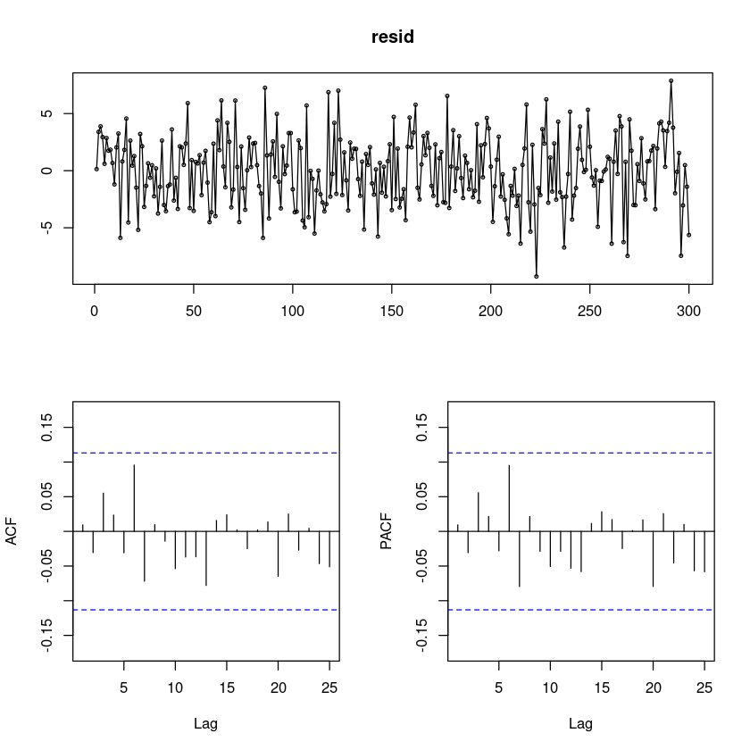
# 잔차의 포트맨토 검정 ## H0 : rho1=...=rho_k=0
portes::LjungBox(fit, lags=c(6,12,18,24))| lags | statistic | df | p-value | |
|---|---|---|---|---|
| 6 | 4.520231 | 5 | 0.4771812 | |
| 12 | 7.964175 | 11 | 0.7165093 | |
| 18 | 10.346863 | 17 | 0.8884381 | |
| 24 | 12.926680 | 23 | 0.9535620 |
## 정규성검정
tseries::jarque.bera.test(resid) ##JB test H0: normal
    Jarque Bera Test

data:  resid
X-squared = 1.1606, df = 2, p-value = 0.5597par(mfrow=c(1,2))
hist(resid)
qqnorm(resid, pch=16)
qqline(resid)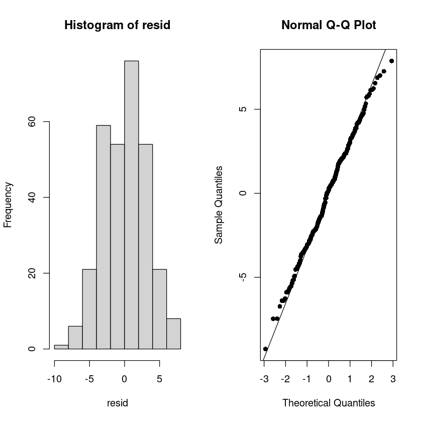
## 잔차 검정
astsa::sarima(z, p=0, d=1, q=1)
initial value 1.355425
iter 2 value 1.182804
iter 3 value 1.144176
iter 4 value 1.129179
iter 5 value 1.127095
iter 6 value 1.125914
iter 7 value 1.125753
iter 8 value 1.125727
iter 9 value 1.125726
iter 10 value 1.125726
iter 11 value 1.125726
iter 11 value 1.125726
final value 1.125726
converged
initial value 1.125981
iter 2 value 1.125979
iter 3 value 1.125977
iter 4 value 1.125975
iter 5 value 1.125974
iter 6 value 1.125974
iter 6 value 1.125974
final value 1.125974
converged$fit
Call:
arima(x = xdata, order = c(p, d, q), seasonal = list(order = c(P, D, Q), period = S),
xreg = constant, transform.pars = trans, fixed = fixed, optim.control = list(trace = trc,
REPORT = 1, reltol = tol))
Coefficients:
ma1 constant
0.7605 -0.0146
s.e. 0.0342 0.3130
sigma^2 estimated as 9.479: log likelihood = -760.93, aic = 1527.86
$degrees_of_freedom
[1] 297
$ttable
Estimate SE t.value p.value
ma1 0.7605 0.0342 22.2124 0.0000
constant -0.0146 0.3130 -0.0468 0.9627
$AIC
[1] 5.109891
$AICc
[1] 5.110027
$BIC
[1] 5.14702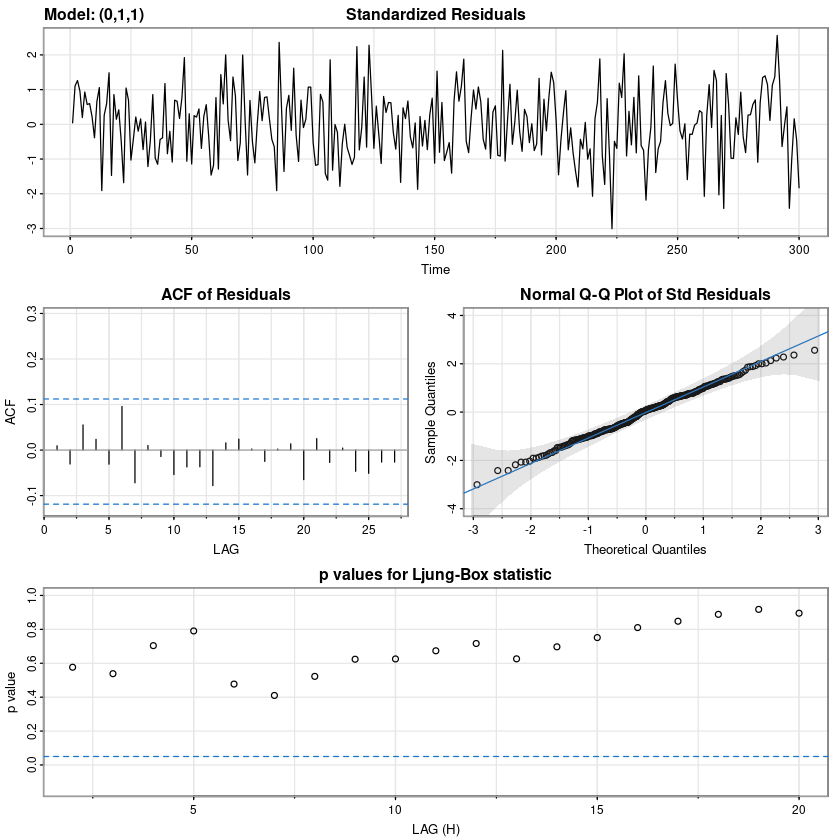
\((1-B)\hat Z_n (l) = \hat \mu - \hat \theta \hat \epsilon_n: l=1\)
\(\hat \mu: l \geq 2\)
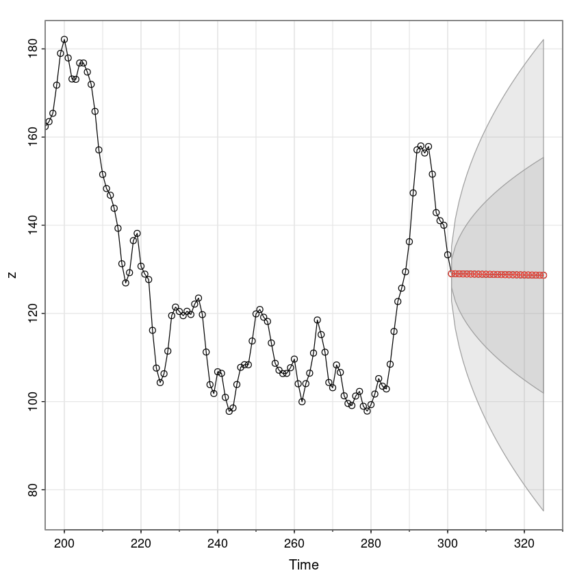
- 원데이터를예측하는 거니까 원데이터 넣어주기(차분데이터X)
fore_fit <- forecast::forecast(fit, 25)
fore_fit
Point Forecast Lo 80 Hi 80 Lo 95 Hi 95
301 129.0191 125.07348 132.9647 122.98480 135.0534
302 129.0191 121.03051 137.0077 116.80160 141.2366
303 129.0191 118.43291 139.6053 112.82893 145.2093
304 129.0191 116.35746 141.6807 109.65480 148.3834
305 129.0191 114.57726 143.4609 106.93221 151.1060
306 129.0191 112.99361 145.0446 104.51022 153.5280
307 129.0191 111.55296 146.4852 102.30694 155.7313
308 129.0191 110.22240 147.8158 100.27203 157.7662
309 129.0191 108.98000 149.0582 98.37194 159.6663
310 129.0191 107.81025 150.2279 96.58297 161.4552
311 129.0191 106.70173 151.3365 94.88763 163.1506
312 129.0191 105.64572 152.3925 93.27261 164.7656
313 129.0191 104.63541 153.4028 91.72746 166.3107
314 129.0191 103.66532 154.3729 90.24384 167.7944
315 129.0191 102.73101 155.3072 88.81493 169.2233
316 129.0191 101.82878 156.2094 87.43509 170.6031
317 129.0191 100.95554 157.0827 86.09959 171.9386
318 129.0191 100.10867 157.9295 84.80441 173.2338
319 129.0191 99.28591 158.7523 83.54611 174.4921
320 129.0191 98.48531 159.5529 82.32170 175.7165
321 129.0191 97.70517 160.3330 81.12858 176.9096
322 129.0191 96.94400 161.0942 79.96448 178.0737
323 129.0191 96.20049 161.8377 78.82736 179.2108
324 129.0191 95.47344 162.5648 77.71544 180.3228
325 129.0191 94.76183 163.2764 76.62712 181.4111plot(fore_fit)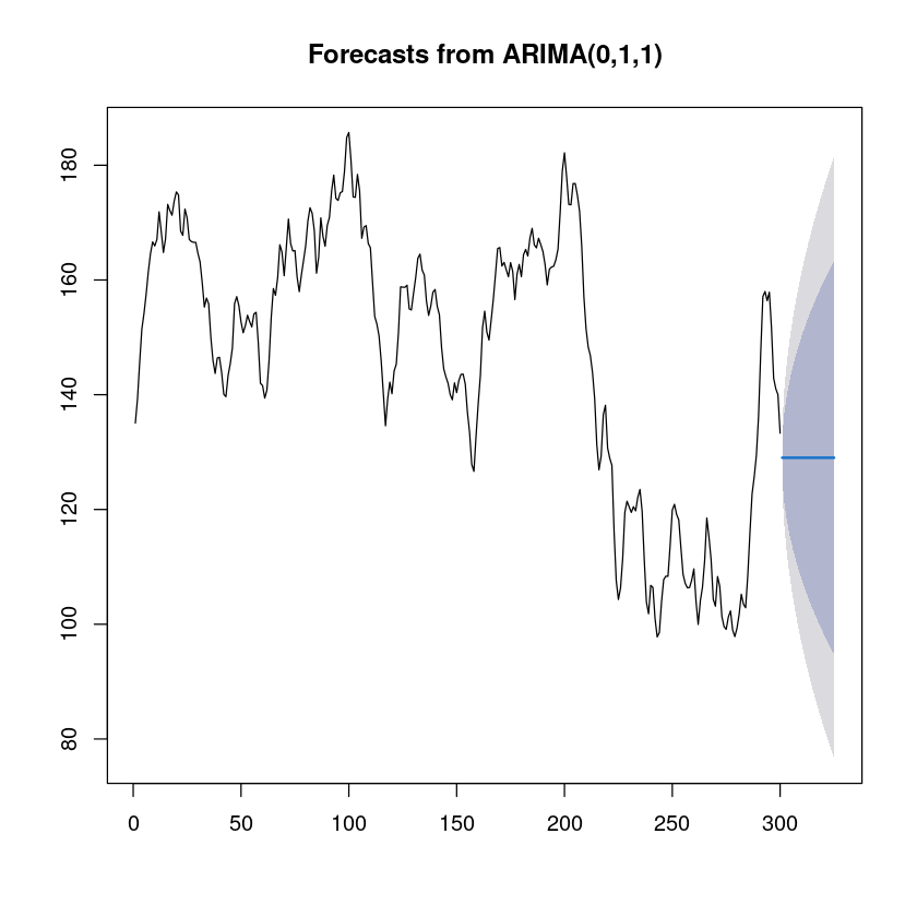
- 평균으로 거의 예측이 됨.
astsa::sarima.for(z, 25, 0,1,1)- $pred
- A Time Series:
- 129.010634626429
- 128.995997383896
- 128.981360141362
- 128.966722898829
- 128.952085656296
- 128.937448413762
- 128.922811171229
- 128.908173928696
- 128.893536686162
- 128.878899443629
- 128.864262201096
- 128.849624958562
- 128.834987716029
- 128.820350473496
- 128.805713230962
- 128.791075988429
- 128.776438745896
- 128.761801503362
- 128.747164260829
- 128.732527018296
- 128.717889775762
- 128.703252533229
- 128.688615290696
- 128.673978048162
- 128.659340805629
- $se
- A Time Series:
- 3.07876798320946
- 6.23357705966339
- 8.26051775756748
- 9.88002147201177
- 11.2691390510429
- 12.5048856698518
- 13.6290438505565
- 14.6672937839507
- 15.6367572600282
- 16.5495271314128
- 17.4145203476207
- 18.2385358404128
- 19.0268983354184
- 19.7838704739663
- 20.5129276700085
- 21.2169477602064
- 21.898345666366
- 22.5591713852255
- 23.2011828201129
- 23.8259009256026
- 24.434652147738
- 25.0286015639165
- 25.6087790983797
- 26.1761005035879
- 26.7313843307499
astsa::sarima.for(lag_z, 25, 0,0,1)- $pred
- A Time Series:
- -4.29136464101854
- -0.014636625581003
- -0.014636625581003
- -0.014636625581003
- -0.014636625581003
- -0.014636625581003
- -0.014636625581003
- -0.014636625581003
- -0.014636625581003
- -0.014636625581003
- -0.014636625581003
- -0.014636625581003
- -0.014636625581003
- -0.014636625581003
- -0.014636625581003
- -0.014636625581003
- -0.014636625581003
- -0.014636625581003
- -0.014636625581003
- -0.014636625581003
- -0.014636625581003
- -0.014636625581003
- -0.014636625581003
- -0.014636625581003
- -0.014636625581003
- $se
- A Time Series:
- 3.07876823197791
- 3.86796612789283
- 3.86796612789283
- 3.86796612789283
- 3.86796612789283
- 3.86796612789283
- 3.86796612789283
- 3.86796612789283
- 3.86796612789283
- 3.86796612789283
- 3.86796612789283
- 3.86796612789283
- 3.86796612789283
- 3.86796612789283
- 3.86796612789283
- 3.86796612789283
- 3.86796612789283
- 3.86796612789283
- 3.86796612789283
- 3.86796612789283
- 3.86796612789283
- 3.86796612789283
- 3.86796612789283
- 3.86796612789283
- 3.86796612789283
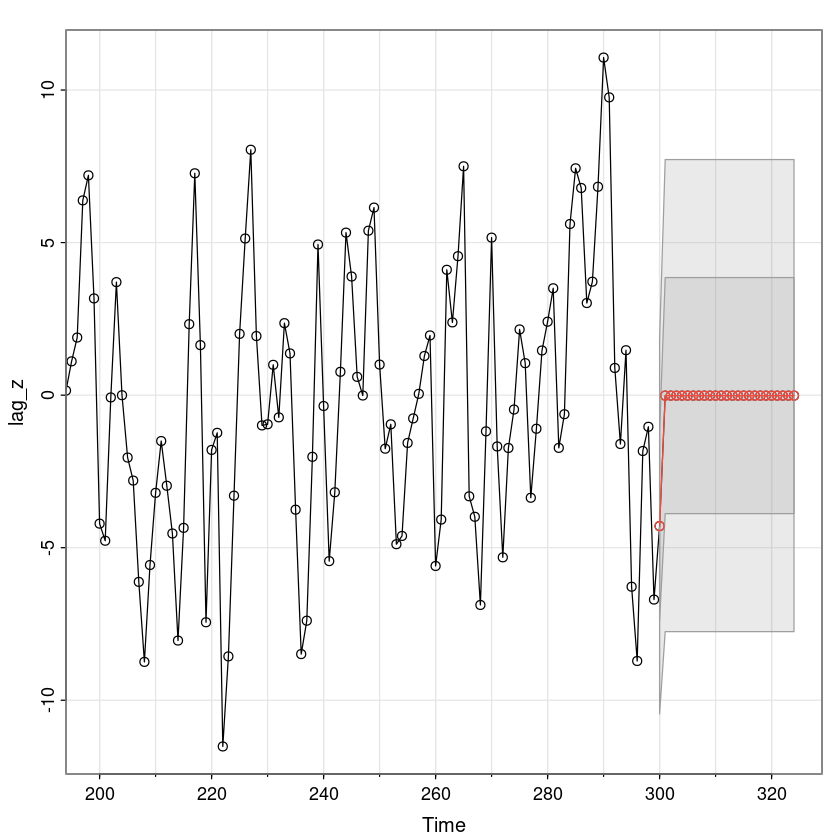
fore_diff_z <- astsa::sarima.for(lag_z, 25, 0,0,1, plot=F)$pred
fore_diff_z
A Time Series:
- -4.29136464101854
- -0.014636625581003
- -0.014636625581003
- -0.014636625581003
- -0.014636625581003
- -0.014636625581003
- -0.014636625581003
- -0.014636625581003
- -0.014636625581003
- -0.014636625581003
- -0.014636625581003
- -0.014636625581003
- -0.014636625581003
- -0.014636625581003
- -0.014636625581003
- -0.014636625581003
- -0.014636625581003
- -0.014636625581003
- -0.014636625581003
- -0.014636625581003
- -0.014636625581003
- -0.014636625581003
- -0.014636625581003
- -0.014636625581003
- -0.014636625581003
fore_diff_z_ <- forecast::forecast(fit1, 25)
fore_diff_z_$mean  # 차분한 값에 대한 예측
A Time Series:
- -4.28290139590614
- 0
- 0
- 0
- 0
- 0
- 0
- 0
- 0
- 0
- 0
- 0
- 0
- 0
- 0
- 0
- 0
- 0
- 0
- 0
- 0
- 0
- 0
- 0
- 0
fore_z <- astsa::sarima.for(z, 25, 0,1,1, plot=F)$pred
fore_z
A Time Series:
- 129.010634626429
- 128.995997383896
- 128.981360141362
- 128.966722898829
- 128.952085656296
- 128.937448413762
- 128.922811171229
- 128.908173928696
- 128.893536686162
- 128.878899443629
- 128.864262201096
- 128.849624958562
- 128.834987716029
- 128.820350473496
- 128.805713230962
- 128.791075988429
- 128.776438745896
- 128.761801503362
- 128.747164260829
- 128.732527018296
- 128.717889775762
- 128.703252533229
- 128.688615290696
- 128.673978048162
- 128.659340805629
fore_z_ <- forecast::forecast(fit,25)
fore_z_$mean
A Time Series:
- 129.01909823039
- 129.01909823039
- 129.01909823039
- 129.01909823039
- 129.01909823039
- 129.01909823039
- 129.01909823039
- 129.01909823039
- 129.01909823039
- 129.01909823039
- 129.01909823039
- 129.01909823039
- 129.01909823039
- 129.01909823039
- 129.01909823039
- 129.01909823039
- 129.01909823039
- 129.01909823039
- 129.01909823039
- 129.01909823039
- 129.01909823039
- 129.01909823039
- 129.01909823039
- 129.01909823039
- 129.01909823039
- 차분한 값에.. 원래데이터의 예측값을 알고 싶다면?
\(\widehat{▽Z_t} = \hat Z_t − \hat Z_{t−1}\)
\(\hat Z_t = \widehat{▽Z_t} + \hat Z_{t−1}\)
\(\hat Z_{300}(1) = \widehat{▽Z_{300}(1)} + Z_{300}\)
z_300_1 <- as.numeric(fore_diff_z[1]) + z[300]
z_300_1
129.010635358981
\(\hat Z_{300}(2) = \widehat{▽Z_{300}(2)} + \hat Z_{300}(1)\)
z_300_2 <- fore_diff_z[2] + z_300_1
z_300_2
128.9959987334